Think Excel Can’t Handle PDEs? Think Again: A Chemical Engineering Case Study

Did you know you can solve 2D partial differential equations (PDEs) in Excel without resorting to macros?

In this post, we’ll look at how to solve Laplace’s Equation, $\nabla^2 f = 0$ , in two dimensions using nothing but Microsoft Excel.

Introduction

Heat transfer is a critical concept in chemical engineering, as engineers often need to design equipment for heating large volumes of potentially hazardous chemicals. Accurate analysis of heat distribution is crucial to prevent overheating and explosions.

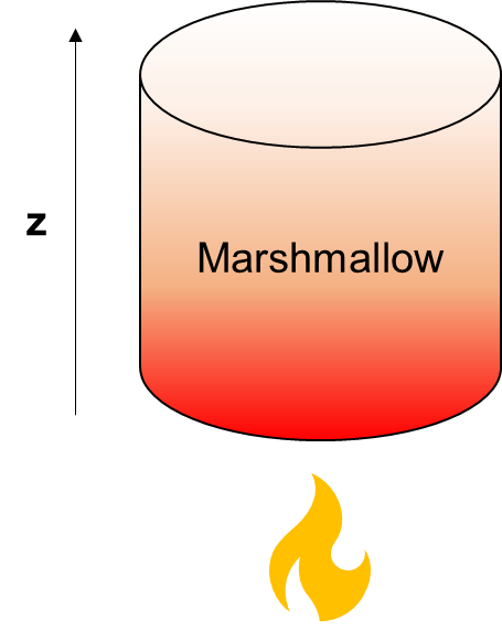
What exactly does Laplace’s equation tell us about heat transfer? Well, one thing it can tell us is what the stable temperature profile of an object will look like after being exposed to a constant heat source for a long time. For example, if you very gently heat a marshmallow from the bottom (making sure that it doesn’t melt or burn!) and hold it there for a while, the temperature will eventually reach a stable profile as heat enters the marshmallow from the bottom and leaves from the sides of the marshmallow. This final temperature profile might look something like this:

The goal of Laplace’s equation is to find a formula that describes this steady state profile (in the case of the marshmallow, $f(z)$ ).

Laplace’s equation in two dimensions

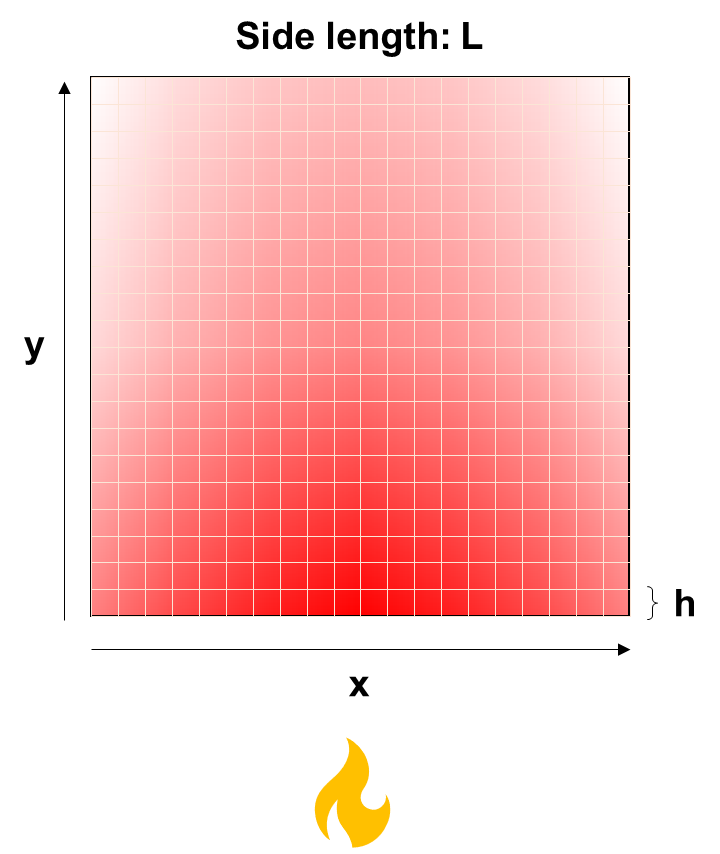
In the example above, I decided to describe the heat profile as only a function of $z$ , the vertical distance from the flame. But in reality, the steady state heat profile might vary both in the radial and vertical dimensions.

To illustrate Laplace’s equation in two dimensions, let’s consider a square plate of metal that we heat on one side, like the one below:

What if we plotted the steady-state heat profile in this plate? It will probably look something like this:

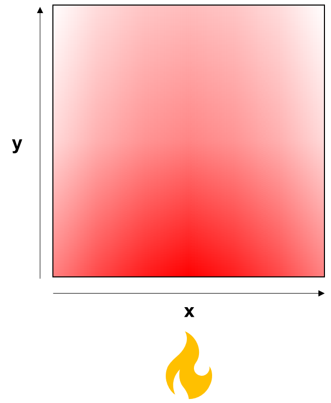
We can immediately make some guesses about what the temperature profile of the plate, expressed as $f(x,y)$ , will look like:

$f(x,y)$ will decrease as $y$ increases: heat dissipates as you get further away from the flame.
$f(x,y)$ will be lowest at the non-heated edges of the plate, since heat dissipates from the non-heated edges.

If we want to explicitly solve for $f(x,y)$ , we can use Laplace’s equation to set up the following PDE:

$\displaystyle \nabla^2 f = 0$

which expands to

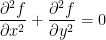
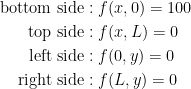
$\displaystyle \frac{\partial^2 f}{\partial x^2} + \frac{\partial^2 f}{\partial y^2} = 0$

We cannot solve this equation unless we also provide a set of boundary conditions. To create a toy model of the plate-heating scenario so that we can solve for $f(x,y)$ , let’s assume that we can maintain the heated side of the plate at $100^\circ C$ and the other three sides at $0^\circ C$ . If we set the origin as the bottom left of the plate and set the length of the plate to $L$ , our boundary conditions are:

$\displaystyle \begin{aligned}\text{bottom side}&:f(x,0)=100\\ \text{top side}&:f(x,L)=0\\ \text{left side}&:f(0,y)=0\\ \text{right side}&:f(L,y)=0\end{aligned}$

Numerical solution to Laplace’s equation

The PDE we specified above is very hairy to solve analytically, so we choose to take a numerical approach instead. One possible approach is creating a coarse grid of points with spacing $h$ and solving for the numerical value of $f(x,y)$ at each point.

We can actually solve for the value of $f$ at each grid point all at once using a clever trick. To do this, we need to assume that each grid point’s value can be inferred from its neighbors’ values. If we can write a linear equation relating these values together, then we can have a separate linear equation for every grid point. So if we have $N$ grid points, we have $N$ linear equations, which we can solve simultaneously!

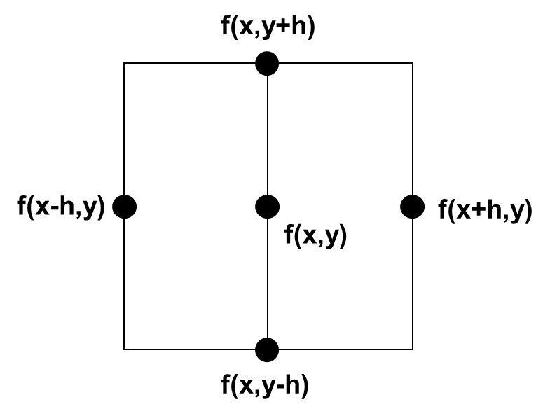
Thus, our task now is to find a linear equation that relates grid points to their neighbors. One possible way to do this is through expansions inspired by the definition of the derivative:

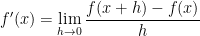
$\displaystyle f'(x) = \lim_{h\to 0} \frac{f(x+h)-f(x)}{h}$

As you’ll notice in this expansion, the derivative of a function can be expressed as the slope of $f$ between positions $x$ and $x+h$ . This can inspire us to write a forward-difference approximation:

$\displaystyle f'(x) \approx \frac{f(x+h)-f(x)}{h}$

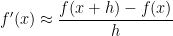
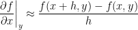
Note: In the above equation, I’m actually being messy with notation since I’ve only written it for one dimension, $x$ . The “proper” way to express this same statement for our 2D grid is as follows:

$\displaystyle \left. \frac{\partial f}{\partial x} \right|_y \approx \frac{f(x+h,y)-f(x,y)}{h}$

It’s not set in stone that we must do a “forward” difference by finding the slope between $x$ and $x+h$ . We can calculate a more accurate derivative numerically by using a central difference between $x-\frac{h}{2}$ and $x+\frac{h}{2}$ , which we express as:

$\displaystyle f'(x)\approx \frac{f(x+\frac{h}{2})-f(x-\frac{h}{2})}{h}$

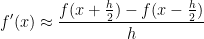
What if we wanted to find the second derivative? We can do this by applying the central difference formula again:

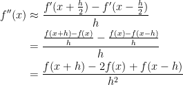
$\displaystyle \begin{aligned} f''(x) &\approx \frac{f'(x+\frac{h}{2})-f'(x-\frac{h}{2})}{h} \\ &= \frac{\frac{f(x+h)-f(x)}{h}-\frac{f(x)-f(x-h)}{h}}{h} \\ &= \frac{f(x+h)-2f(x)+f(x-h)}{h^2} \end{aligned}$

Using this, we come up with the following approximations for the terms in Laplace’s equation:

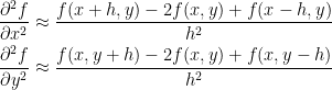
$\displaystyle \begin{aligned} \frac{\partial^2 f}{\partial x^2} & \approx \frac{f(x+h,y)-2f(x,y)+f(x-h,y)}{h^2} \\ \frac{\partial^2 f}{\partial y^2} & \approx \frac{f(x,y+h)-2f(x,y)+f(x,y-h)}{h^2} \end{aligned}$

Substituting into Laplace’s equation, $\frac{\partial^2 f}{\partial x^2}+\frac{\partial^2 f}{\partial y^2}=0$ , we get

$\displaystyle \frac{f(x+h,y)-2f(x,y)+f(x-h,y)}{h^2} + \frac{f(x,y+h)-2f(x,y)+f(x,y-h)}{h^2} = 0$

which simplifies to

$\displaystyle f(x+h,y)+f(x-h,y)+f(x,y+h)+f(x,y-h) - 4f(x,y)=0$

Solving for $f(x,y)$ , we get

$\boxed{f(x,y)=\frac{f(x+h,y)+f(x-h,y)+f(x,y+h)+f(x,y-h)}{4}}$

In other words, each cell is the average of its neighbors. If we have $N$ interior grid points and $M$ grid points on the boundary, we can start writing a system of linear equations to solve for the $N$ interior grid point values. For notation’s sake, let’s call each temperature value on the grid $T_{i,j} =f(x_i,y_j)$ . Then our $N$ interior equations will have the form

$\displaystyle T_{i,j}=\frac{T_{i+1,j}+T_{i-1,j}+T_{i,j+1}+T_{i,j-1}}{4}$

while our $M$ boundary points are given values $T_{i,j} = C_{i,j}$ , which we obtain from our boundary value problem’s specification. Since we now have a set of $N$ equations with $N$ variables, and we can solve for the temperature profile by solving all $N$ equations simultaneously.

Using Excel to solve Laplace’s equation

Solving all $N$ equations simultaneously can require a lot of memory, which is a problem. If our grid contains a total of $N=n^2$ interior points (where $n$ is the side length of the grid, excluding edges), we will obtain $n^2$ equations. Then if we naively plug this into a linear equation solver, we would have to express these equations as an $N \times N$ matrix of coefficients (one row per equation), which contains $n^4$ values.

If we want to avoid this, we might try an iterative method instead, where we just work directly on our grid of $n^2$ values. The idea behind this is to load our initial guesses into the grid, and then nudge the values around until they satisfy Laplace’s equation.

In the case of Laplace’s equation, we can nudge the values around by repeatedly applying the averaging formula we derived earlier to every grid point, and just hope that we get a stable solution.

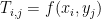
Let’s try this in Excel. What we’re going to do is initialize the interior points with an initial value of 0 and set the boundary value to 100 on the bottom of the plate (I’ve used conditional formatting here to make higher values red):

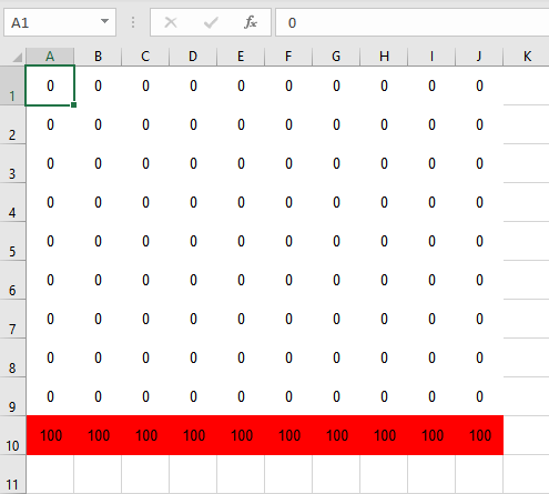
Next, we’ll input our averaging formula into the top left interior cell, and use Excel’s click and drag feature to copy the formula to the rest of the interior cells:

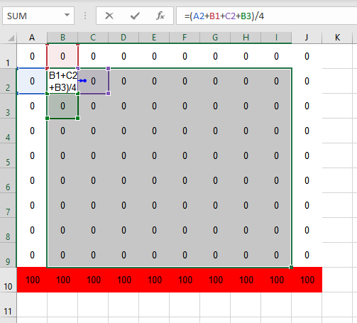
Our interior values haven’t changed! Why? Because we have circular references, which Excel refuses to operate on. The value of cell B2 depends on the value of cell C2, but the value of cell C2 depends on the value of B2. To get around this, Excel has an option for iterative calculation, under Options -> Formulas -> Enable iterative calculation.

Let’s enable it and see what happens:

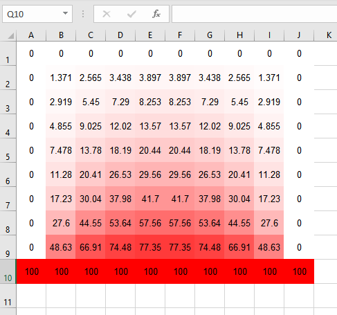
Amazingly, this converges! This should be surprising because everything about our implementation so far has been sloppy – we kind of threw our derivative approximations at Excel, asked it to repeatedly update the values at each grid point based on these equations, and crossed our fingers hoping that this process would converge. It’s not immediately clear why this would be numerically stable, so let’s examine why this is the case.

Analysis of numerical stability for Excel method

It turns out that what we’ve done is secretly equivalent to the Gauss-Siedel method for iteratively solving matrix equations. If we chose to solve the system using the Gauss-Siedel method instead of the Excel method outlined above, we’d have to construct an $n^2 \times n^2$ matrix $A$ representing the equations for our interior point temperatures and perform updates to a length- $n^2$ solution vector $x$ until we achieve the solution, $Ax=b$ . These updates work by separating $A$ into its lower triangular slice $L$ and its strictly upper triangular slice $U$ , and updating $x$ using the formula $x_{new} = -L^{-1}(b-U x_{old})$ . What this formula does is the equivalent of iterating through each equation $i$ in our system, solving for $x_i$ in terms of $x_{j \neq i}$ , and updating $x$ with the new value of $x_i$ before moving on to the next equation.

In our Excel implementation, this is indeed what we are doing when we repeatedly apply our averaging formula: we express each element of $x_i$ in terms of other elements of $x$ , update the value in place, and move on to the next value. Since Excel executes iterated calculations from left to right, top to bottom, it performs the Gauss-Siedel iteration the same way each time it goes through the entire matrix.

Why does our implementation converge? The Gauss-Siedel method is guaranteed to converge for strictly diagonally dominant systems, or systems where the magnitude of all diagonal elements of $A$ are strictly greater than the sum of the magnitude of all other entries in the same row, i.e.,

$\displaystyle \forall i, |a_{ii}| > \sum_{j \ne i} |a_{ij}|$

In the case of our averaging formula, $T_{i,j}=\frac{1}{4}(T_{i+1,j}+T_{i-1,j}+T_{i,j+1}+T_{i,j-1})$ , the diagonal elements of $A$ (i.e., the variables we are solving for) will have a magnitude $1$ (i.e., the coefficient of $T_{i,j}$ ) and the four off-diagonal elements will have magnitude $1/4$ (i.e., the other coefficients in the equation). Our convergence criterion is not met since the diagonal elements have magnitudes that are equal to the sum of the magnitudes of the off-diagonal elements: $1 = \frac{1}{4} + \frac{1}{4} + \frac{1}{4} + \frac{1}{4}$ . Thus, the Gauss-Siedel method is not guaranteed to converge for $A$ . However, if we provide reasonable initial conditions, it is still possible for the method to converge – it just isn’t guaranteed.